Glance puts content on the lock screens of millions of phones. A lot of that content is news, and that comes from many publishers who post to Glance. Stories need images, which at Glance means wallpapers. Most publisher images wouldn’t fit the high quality and size requirements of full-screen wallpaper. Even if they did, we probably don’t have permission to use them. And most stories don’t come with one at all.
So for every story, we need an image that we are actually allowed to use and that meets our spec. Licensing a fresh image for each story is expensive. The cheaper way is to reuse images we have already licensed over the years and edited to our specs. That’s where our image search system sits. The task is simple. Out of a library of millions of already-licensed, spec-ready images, find the one that matches this story
In early 2021, the system in place was based on tags. We would use expensive image APIs to tag images as we ingested them, then matched those tags at search time with a simple SQL query on Postgres. But over time the system had built up so many tags which were in inconsistent formats and had varying quality, that the search was taking over 90 seconds to comb through the database and still return results that in the end were replaced by a human.
The motivation was the complaints from editors. The “auto” publishing flow would require too many interventions from the editors, the support channel for the system was filled with issues of image search.
Two kinds of queries
The system gets queried from two quite different places. The first is automatic publishing. When a post comes in, the publishing system auto-selects an image for it, and in that case “query” is just the article’s title and description. This is the most used path and the queries are not compositional and just a news story title.
The second is a human typing a query by hand. This happens when they did not like the auto-selected image and want to pick a different one, or when they are publishing brand new article and didn’t come from automatic workflow. This is where the queries get specific, like a caption to an exact picture in their head.
How should we build it?
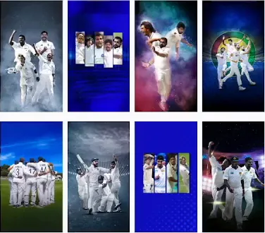
Should we just improve the tag-based system? Maybe a better API? more consistent tags? or a more expressive tags API maybe? maybe we cleanup some of the noisy tags? or make a weighted tag matching by TF-IDF (i.e. rarer tags contain more information)? All seem like good ideas. In this system the quality of a search was only ever as good as the tags, and the tags could never cover the long tail of all the details in the picture. For example, searching “cricketers” might work, “cricketers in white jersey” will not, because almost no API tags the jersey color.
And even if we build the best tags system, how do we solve the latency issue? This was the motivation to build a semantic vector search. But at the same time we needed immediate fixes until this semantic system could be built. So we invested in both.
Building a semantic search
What semantic search is
A keyword search matches the words in your query against the words (here, the tags) attached to each image. A semantic search matches meaning. If you search “a cricketer celebrating”, you want the right photo back even when its tags say nothing about celebrating: the words don’t overlap, but the meaning does. So the goal shifts from “which words do the query and the image share” to “how close is what they mean”.
My experience with systems like this was in text, i.e. to calculate similarity between different texts. Rather than matching texts by words, we embed them into vectors and take cosine similarity to match them. If I want to build it for images, I could embed images into embeddings, and match with other images and find the most similar ones. But our input is text. If somehow I could convert the input text into an embedding that’s similar to an image embedding, then the problem is solved.
The two-tower model
The two-tower idea comes from recommendation systems. At Glance, recommendation is our bread and butter so we had some understanding of this type of system. The main reference for us was Google’s YouTube retrieval paper. You have two separate neural networks, the two “towers”. One encodes the query (in YouTube’s case the user and context), the other encodes the candidate (a video). Each tower outputs a vector, and the towers are trained together so that a matching query-candidate pair lands close in that shared latent space and a non-matching pair lands far apart. Then to recommend content all you have to do is embed the “user”(query) and find all the nearest contents in the latent space (candidates).
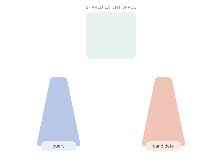
In our case, the query would be the article title and description, and the candidate would be the images.
Training the towers
How do you actually train it so that matching pairs get a high dot product? The YouTube paper frames it as extreme multiclass classification: every candidate in the corpus is its own class, so you are classifying among millions of classes. Given a query embedding, which candidate out of the entire corpus is the right one? That is a softmax over all candidates:
$$P(w_t = i \mid U, C) = \frac{e^{v_i u}}{\sum_{j \in V} e^{v_j u}}$$$u$ is the query embedding (from the query tower) and the $v_j$ are the candidate embeddings (the image vectors, from the image tower), and $V$ is the corpus of candidates. The term in the exponent, $v_i u$, is just the dot product between the query vector and a candidate vector, which is their similarity. Training maximizes the probability of the correct candidate, so it essentially maximizes the dot product.
We had about 3 million image and title pairs. Now, obviously we cannot fit all the candidates in memory during training, so instead we do softmax on all candidates in a batch.
We built and trained the towers with TensorFlow Recommenders (TFRS), TF’s official library for recommendation system models.
One detail on the negatives: TFRS generally suggests hard negative mining, but we used a simpler variant and skipped it. We just treat every other pair in the batch as a negative, plain in-batch negatives. So within a batch, each pair is the one positive against itself and a negative against all the rest, which makes the loss symmetric: every image is pushed away from the other titles, and every title away from the other images.
Bootstrapping the towers
Are 3 million image-text pairs enough to train a fully semantic image search? I didn’t think so; these are news stories and their titles. “These are a very specific distribution of images and text. So it probably would not cover a lot of semantic concepts especially for the human editor queries. I did give it a try; the training took forever.
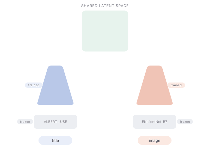
So instead of training the towers from nothing, I bootstrapped them with pretrained embeddings on both sides. For images I used EfficientNet-B7. For text I tried ALBERT and USE (the Universal Sentence Encoder) across different experiments.
These embeddings already have a lot of important information of the images and the text, so the idea is to use neural networks on top to effectively translate from one latent space to a shared latent space.
The result genuinely did semantic search. I tried lots of queries like “desert”, or “desert at night”, returned the right images even though no one had tagged them that way. But it had a major flaw, a specific failure mode: proper nouns. Search for a specific person’s name or place name and it fails to bring up matching images. This could be coming from two places. One, the name is unique enough that the tokenizers of the input embedding models have never seen it, so, the embedding itself has no information about the person or the place or it could be from failure to convert this specific information into the shared latent space as they are so rare in the training data. This could potentially be fixed by augmenting the training data.
By this time we had some improvements on our tag-based system, Shiv had built a faster keyword search using Typesense (v0.20 at the time), which is fast and typo-tolerant but back then had no notion of semantic meaning. So we bolted that on alongside the semantic model to cover the proper-noun gap. Basically combine results from both and prefer keyword search results when query is one or two words and semantic search when it’s longer and more complex.
CLIP and contrastive learning
OpenAI’s CLIP paper came out in early 2021, and we came across it around the time we released the hybrid two-tower search. I had just spent a while looking for a bigger training set and had landed on YFCC100M, and CLIP came already trained on 400 million image-text pairs, two orders of magnitude more than our 3 million.
CLIP (Contrastive Language-Image Pretraining) is the same two-tower setup we had built: an image encoder and a text encoder that map into one shared latent space.
The loss function itself is pretty similar to ours, with two small changes. First, CLIP L2-normalizes both vectors before the dot product, so the similarity is a clean cosine similarity between [-1, 1] rather than a raw dot product that can have any value. Second, it multiplies those cosine similarities by a learned temperature parameter, that controls how sharply the softmax differentiates the similar and dissimilar pairs.
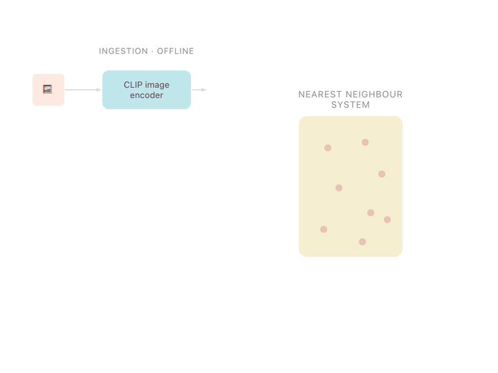
Because the architecture matched, CLIP dropped straight into our pipeline. We swapped our towers for CLIP’s encoders and kept everything else. Offline, every image in the library runs through CLIP’s image encoder once and its vector goes into the index. Online, the search text runs through the text encoder and we return the nearest image vectors.
The one issue was the input image resolution. The model weights that were out at the time were the small RN50, which takes 224x224 inputs, and our images are 16:9 and much higher resolution, so squeezing them into a 224 square meant heavy black padding and worse quality matches. Luckily the RN50x16 weights landed soon after, taking 336x336 inputs, which gave us more pixels and better results.
One thing to notice is, there is nothing stopping us from using image encoder in query time to perform semantic image to image search, and we did implement it as a feature in later releases.
Finding the nearest vectors fast
A naive nearest-neighbour search scales linearly with the number of images in the pool. The more images we add over time, the slower each search gets, since we have to calculate a dot product against every one of the images. In our case that is 3 million dot products per search, which is very expensive. So we trade off some accuracy for speed using an Approximate Nearest Neighbours (ANN) search instead.
Instead of checking every image, ANN algorithms build an index ahead of time that lets you find the most of the closest vectors while only looking at a small fraction of them. To illustrate how this is possible, let’s take a simple index based on clustering. We take our pool of images, convert them to embeddings, and cluster them into K clusters. Now when we want to search, we embed the text and match against the centroids. Then we only match against the vectors inside the nearest cluster (or the few nearest) by centroid similarity.

This is very simplified. Real ANN libraries layer on a lot more, smarter indexing structures, quantization to shrink the vectors, multiple probes to recover accuracy, and so on, all to make it genuinely fast while limiting the downsides of approximating. There are many existing libraries for this, like Annoy, Faiss, etc. We used ScaNN, Google’s ANN library, mainly because we were on GCP and got it out of the box rather than having to deploy and manage our own. And it is one of best on the ANN benchmarks.
Results
Offline, while experimenting, we used Recall@K and Precision@K, where K is the number of images we return as results. Precision@K is: of the K images we showed, how many were actually relevant. Recall@K is: of all the relevant images in the pool, how many did we catch in the top K. In our case the test dataset was the image-text pairs, so the value can only be either 0 or 1, 0 when the image is not surfaced in the top K results for its text, and 1 when it is. So we can aggregate these metrics across the whole test dataset.
In production, we tracked three metrics:
- Auto-select quality. For the automatic path, how often did a publisher edit the auto-selected image? Every edit is the system having picked something the human did not want. The lower the human edit rate better the model is doing
- Search sufficiency. When the humans do update, how often is it a brand new image instead of a search result. This means all the images we surfaced were not good enough.
- Latency. the time taken to surface the results.
These two production metrics map well to our offline metrics. Auto-select shows the very top of the results, so the override rate is is precision@1. Search sufficiency is Recall@K: when a usable image exists in the library, the publisher picks from the results only if search actually surfaced it in the K results they looked at. There is an upper bound to the improvements we could do on these metrics as there will be genuine missing image cases, our pool doesn’t contain all the images that could be needed only the images we have used in the past.
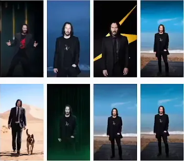
The share of auto-selected images a publisher felt the need to manually change came down by more than half. Even when a publisher did go and search by hand, it was very rare that they had to license a brand-new image. The typical latency of the system was less than 100ms.
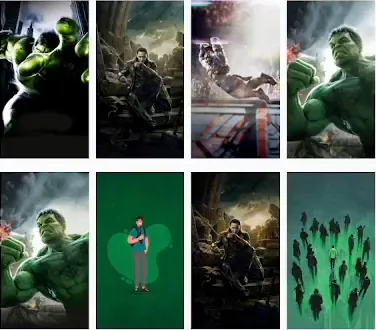
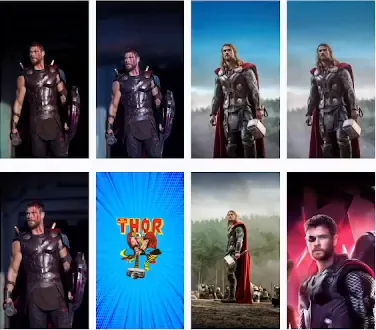
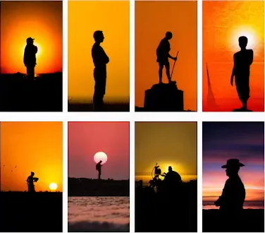
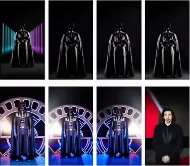
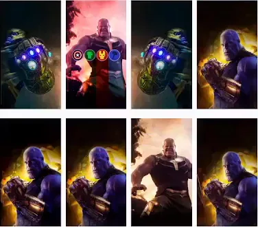
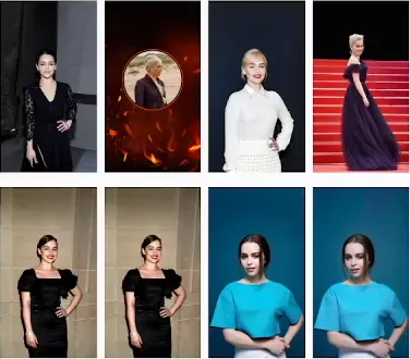
“cricketers in white jersey” “that green dude from avengers” “the guy with a hammer in avengers” “a silhouette of a man with sun setting in the background” “You’re Breathtaking” “No, I am your father” “I am inevitable” “mother of dragons”Fun queries we demoed